The scribe... kinda

Hello there. Van scribing for Monday's class. Not much happened. Substitute teacher gave us a worksheet to hand in for Wednesday's class, and it's worth 100 marks each, 5 questions total.

That's about it.

Next scribe... Dino...

The Return of the Lost Scribe... whoops

So now we are well into exam review and for good reason. (There are only 6 classes left until the exam).

On Thursday our class consisted of five accumulation problems from the AP exams of five different years.

We completed them in groups and then Mr. K. went over them in class. The questions were not extremely hard, but there were a few tricky parts. I believe after Mr. K. discussed them in full, we understood where we had made our mistakes.

The more important part of the exercise was to notice how the same type of problem changed over the different years. Looking at them, you can see that the graphs are the most noticeable things that change. They become less familiar in behaviour and less points are actually drawn and labeled. The graphs also begin to have a lot of corners which are discrepancies in the second derivative as the are undefined. It then asks if these points are points of inflection, which are usually calculated via the second derivative. That is probably the trickiest part of these questions, but with a little understanding of how the derivatives and their graphs relate to each other, it is easy to get around.
The questions also change fairly drastically, as they go from just understanding how to use the graph and the given functions, to looking past the given graph and fuctions and using it to find characteristics of the parent/derivative functions and their graphs. In the later examples, they begin to ask questions about behaviour of the functions over certain intervals and even ask to draw the graph of the parent function on the axes.
The final example (from 2007) is quite different from the others as there is no graph given, but a table of values is. The table includes two functions (ƒ and g) and their derivatives. It then asks questions about the function h(x) = ƒ(g(x)) - 6 and how it behaves over certain intervals. It also asks a new question that we have not seen yet.
It asks us to find the derivative of the inverse of a function ( g^-1 ). It is a rule that Mr. K. has not yet taught us, but it was explained to me as "the derivative of an inverse of a function is equal to the inverse of its derivative" basically, ∂/∂x(g^-1) = 1/g'. From there just apply it as you would any derivative and solve the question.

Finally, Mr. K. said that this last example is probably the closest example of how it will be presented on our exam, so it would be a good idea to go over this some time in the next two weeks to make sure you have this under your belt, it should be easy marks now.

That is all for my scribe post, remember to start studying "fiendishly" (if you haven't already) there are only 18 days left. O_O

The next scribe is Van I guess...

Enjoy the rest of your weekends!

April 15 Post

SCRiBE: Last Of Content

Hello everyone! I'm known as Tim-math-y and I'm the scribe for Thursday's lessons. On Thursday, our topic was: Solving Differential Equations Symbolically and Newton's Law of Cooling.

Introduction:

Solving Differential Equations Symbolically and Newton's Law of Cooling:

On Thursday, we learned more about differential equations, this time using the symbolic (algebraic) approach. This topic tied into Newton's Law of Cooling. According to this law, a hot object cools at a rate proportional to the difference between its own temperature and that of its environment.

By applying this concept, we solved questions that dealt with cooling.

Content and Lessons:

First we began by deconstructing the equation of "dy/dx = ky." Mr. K mentioned in the past that normally, you are not allowed to pull apart the differential operator. However, without going through the complexities of why it is possible, we pulled it apart.

By seperating the two variables, including both 'dy' and 'dx', we found a familiar term that could be antidifferentiated.

Through algebraic play, we found the equation that defined the parent function of cooling.

*Note: the variable "c" and "C" are different in value but generally both represent a constant.

Next we looked at an example question.

• First we assigned variables, F = Temperature in Degrees of F and t = T time in Hours
• Second we applied the variables to "dy/dx=ky" to produce "dF/dt=k(F-20)" where 2o is the lowest temperature the object can attain in an environment
• By applying the same steps to seperate 'dF' and 'dt', we antidifferentiated and worked the out an equation that could be used to find 'F', the temperature, at any given time. The only unknown left is the constant that we have yet to solve.
  

By using the information given (two pieces of data that showed us the temperature at a specific point in time) we substituted the values in and solved for the final equation that represented the temperature at any given time of this situation.

At this point, we considerred both questions solved.

Next, we looked at another example question (Don't be overwhelmed by the length of the question as most of it is just a background story that Mr. K conjured up: The information required is located in paragraph 3).

By applying the same steps from the previous question, we found the solution to the problem. Again, our variable assignments were the same. The only difference is that the coldest temperature in this situation was 25 degrees. We found the equation that still included the constant value of C.

By taking this a step further, we inputted the coordinates given (temperatures at given times) and solved for the value of C to in turn, solve for the final equation.

Finally, by inputting the temperature of the cola at an unknown point in time, we solved for the uknown value of 't'.

Conlusion:

We went through two problems that dealt with Newton's Law of Cooling, solving differential equations symbolically.

******

Homework is on the end of the slides posted in the previous post! Answer is on the following slide.

Tomorrow's Scribe is... Craig!

Happy Easter? Haha, good night.

The Edmonton Eulers Method

Hey everyone, it's MrSiwWy here as the scribe for March 18's class on Euler's method. I know I started this scribe post pretty late, but I just got home from the fashion show at school, which was definitely an enjoyable occasion. I really found this topic quite interesting, so I'll very much enjoy explaining his method as intricately as possible. Now with classes only every second day, I didn't think scribe duties would remain so frequent, though the class is indeed quite minuscule in comparison to the class size first semester. Oh yes, and before I begin, I think i must note that all explanations will be accompanied by an example furthering my explanation in a different text colour. Text in black will be initial explanations, while text in green will pertain to explanations using an example for the first part of the post and text in blue will pertain to explanations using an example for the second part of the post. Hope it works out well. Enjoy!

Scribe
~~~~~~

I can't remember exactly how class started, though I do recall it initiated with the usual abstract chatter and various technological utility exposures by Mr. K. But what I do remember, is beginning the actual lesson with a very fundamentally elegant and quite remarkable equation; Euler's identity.

Though we didn't go in depth into what Euler's identity is and how it was formulated, but we did vaguely discuss the implications of the identity. The sheer elegance of the equation derives from the fact that it contains and also intertwines the destiny of five of the most important constants in mathematics: 0, 1, (pi), i, and e. Euler's identity is as follows:


Now we transitioned into the basis of the day's topic: Euler's method. I think it's quite a useful technique, and is a very innovative technique with easy implementation (at our level at least). We started off with a demonstration of Euler's method without any formal introduction quite yet. This demonstration can be found here. If you follow the link, it might ease the subsequent explanations tremendously.

- First off, imagine that you are given an initial value problem. Recall that an initial value problem is a problem in which you are given a differential equation to solve as usual, but you are also given a point that exists on the parent function/solution to the differential equation.

*In this case, as used by the aforementioned demonstration, take the differential equation to be y'(t) = 1 - t + 4y(t) and the initial point to be y(0) = 1. This means that at t = 0, y(t) = 1. Following the above link will drastically clarify this example. Also, take note that we know the point (0,1) on the differential equation solution, and therefore have an exact solution and not just a general one. A general solution only represents the family of functions that could fit the solution for the differential equation. An exact one means that it's only specific function, and not a whole family.

- Now, there is an important idea that I must stress in order for Euler's method to be utilized easily, so pay attention in case you missed it in class. We must find a way to get another point on the parent function, which can be easily determined by plugging in the initial value/point into the differential equation to solve for the slope of the line tangent to the function at that point. Using this slope we can use our classic definition of slope to yield the next point that exists on the function y(t) given a certain step.

*The point (0,1) is known to lie on the function y(t), but how are we possibly going to get another point on this function? Well, as I stated earlier, since we know the differential equation, we can plug in the point (0,1) into the differential equation (which is y'(t) = 1 - t + 4y(t) in this case) and determine the slope of the line tangent to the function at that point. This is because the differential equation will solve for y'(t), which is the derivative of y(t) or rather the instantaneous rate of change of y(t) at a given t. This is particularly useful since using our rather classic definition of "slope" (rise over run) will yield our next point. By plugging in the initial point into the differential equation as follows, we can determine the required slope:

y'(0) = 1 - (0) + 4(1)
y'(0) = 5

Using this slope with the "old-school" rise over run definition of slope, we can easily determine the next point. But be careful, you must pay careful attention to the steps or the scale of each axis to correctly apply this definition. Since the steps we will be using in this case are 0.1, that means that instead of the function increasing upwards by 5 and increasing rightwards by 1, the function will increase upwards by 0.5 as it travels rightwards by 0.1. This means that the next point will be (0.1, 1.5). Using the next button on the demonstration page will automatically graph the next point on the function.

- Now that we have two points on the graph, we can easily repeat the above process to determine any subsequent points and find an accurate portrayal of the solution. The only problem is that you must use a sufficient amount of steps by decreasing the amount of change along the x-axis (or in this case t) so that each point will be closer to each other and each subsequent derivative will be more accurate than with little points. I advise using this website or this website to help grasp this concept. Review one of these sites to further your understanding of what I have just said. Also, concerning this idea, I tend to think of Euler's method as being quite similar to how an integral works. In an integral, you must let the dx values (or dt) get as close to 0 as possible, so as to increase how accurate the solution truly is or how well the integral fits the actual shape of the function. This is exactly how Euler's method works.

*Each time that you press the next button on the above demonstration, the graph will further the use of Euler's method and graph the next point on the parent function, thereby creating an approximate graph of said function. But notice how choppy each segment looks, even though as a calculus student(and others =p) you should recognize the function to be curved.

Once we were introduced to Euler's method using a bevy of demonstrations and tools to ease the idea of his method to us, we were asked to apply what we had just learned to a problem. This can be seen on the following slide:


In the above slide, all that we really did was find a way (basically on our own) to efficiently repeat the process I detailed above. Though there were some alterations in this problem.

*Basically, when you were given the initial point, you could plug the point into the differential equation (which is y' = y - x this time) to find the derivative of the function at that point. This derivative will be m, or the slope of the tangent line at that point, which can be used by rearranging the m = Δy/Δx equation into Δy = m * Δx. Since m has just been calculated, and Δx (which is the step as I mentioned above) is given in the question as 0.25. Calculating Δy will give us the change in y from the first point to the next point given a certain step, which means we'll know the next points x-coordinate (the first point x-coordinate plus the step) and y-coordinate (the first point's y-coordinate plus the Δy calculated). Thus, this "next" point will be our "initial point" in the next part of the solution. If you use the above slide to help with understanding this idea, then each row will be one iteration of determining the solution to the differential equation. An iteration means a complete round of doing something, such as the process that is being repeated within a loop (which can be taken as the process I detailed above in the first detailed section of this scribe post).

But how can we make this process simpler and reduce the irksomeness of the entire process, especially for cases with a lot more repetitions? One way that we worked out during class involved using the store function in our calculators. This method can actually have several approaches, but basically you can utilize your calculator's store functions in many ways to achieve the same thing. Here's basically what you do:

- Store the initial y value into any variable in your calculator, say A.

- Input this variable into the differential equation on your calculator, and multiply this new expression by the step, and finally add A to this whole thing and store the new answer back into A. It might be hard at first to type this all in within one shot, but it is doable if you do it enough. Below is an example of how it should look in your calculator using the above question.

*Applying this step to the slide above, here's what it would look like in your calculator:
(((A - 0)0.25) + A) -> A

- Simply repeat this line using the [2nd] then [enter] function in your calculator, each time changing the x value according to how the point has changed.

*Again applying this step to the slide above, here's what the next line would look like:
(((A - 0.25)0.25) + A) -> A

Using this method yielded the answers shown in the above slide, which could be taken as solved since the last point on the interval asked for (which was [0,1]) was determined, the question was answered. Though, Mr. K wrote down the exact answer to the problem at the bottom of the slide, which wasn't that close to the answer we arrived at.

So then we tried using more segments to approximate a solution that is much closer than achieved above. We did this by using our new found method of numerically solving initial value problems with Euler's method, we attempted another problem. Though it may look quite empty, all of the work was quickly repeated on our calculators using a method roughly equivalent to the one above, and we all arrived at the same answers as shown in the following slide. I suggest trying it out on your own for some practice. (note: The question is basically the exact same as the first, but it uses far more segments and a much smaller step).


Just before class ended, Mr. K distributed the "EULER" calculator program for us to use to quickly solve problems involving Euler's method.


I will post the algorithms and full code for the program here when I get the full version again, since someone accidentally erased a line in the program and I can't remember what that line was.

Okay, that's all for my scribe for now. I still have some stuff to edit, but it's getting pretty late now and I don't want to be late for Chemistry again tomorrow (I bet people in Chem would doubt that). Anyway, the next scribe will be:
Tim-MATH-y!
Well good night everyone, see you all in class tomorrow! Please just talk to me or comment if there are any questions, complaints, anxieties, confusions, etc. =p Good bye all!

The Pi day scribe

Well, a certainly enjoyable pi day it was. Lots of treats and Friday!. Doesn't get much better than that.

With all the celebrating, we didn't do very much.

We learned, the slope fields were the graphs of the parent function. Just moved all over the place.

Due to my internet moving unbelievably slow, I will add more "pi" pictures when it starts to pick up. (Litterally, 3 minutes to load a single page)

Next scribe.

Mr.SiwWy-chan

Absolutely Late Scribe..... Sorry guys.

WOW! Very, very sorry about the tardiness of this scribe... I worked both last and this evening and today was very busy.

So Wednesday's class started with a very unusual period in which we were given our tests back and allowed 10 minutes to continue them since we didn't get a chance last Thursday.

Then we briefly discussed the Developing Expert Voices projects as Mr. K. handed back the proposals.

Following that was a little conversation about "π day" (which is today actually). I'm bringing either a Strawberry-Mango or Blueberry-Peach pie =D.

Finally we started the lesson for the day. The first thing we did was a quick review of Differential Problems.
It dealt with a set amount of oil in a reserve, states that a function A(t) as the rate of consumption, and provides the derivative of the rate [ A'(t) ]. How long until the reserve is completely emptied.

Basically, to solve it, find the antiderivative, A(t)+C, of the the given function and then plug in t=0 to find the constant (C).
From there it is as simple as finding the positive root of that function and that will be the answer.

Next we moved onto the new content.
SLOPE FIELDS

these are kind of tough to explain... I'll let some pictures speak some of my words.
This is the FIELD in which we plot the SLOPES. Easy enough right?
So we first tried it with the expression ( ∂y/∂x = y ). This means that the derivative of any point in the function is the value of the function at that point (y-coordinate).
•Let's say we want to plot the point (1,1). The derivative (SLOPE) of the function at that point is 1, so we draw a small line with slope 1 at that point.
•Next, take the point (3,2). The derivative at that point is 2, so there's another small line, but with a slope 2 at the point (3,2).
Now, you understand how they are constructed, this is how the SLOPE FIELD of the function(s) that have ( ∂y/∂x = y ).
From here, you can solve for the point (1,1).
To do this, draw a curve that follows the slope of the line in either direction until the next whole number is reached. At that point, change the curve's slope to that of the new poitn and continue until the next whole number and so on... WHAT FUNCTION DOES THE CURVE LOOK LIKE???
Correct! It is easy to see that the function that has a derivative equal to the value of the function and passes through the point (1,1) is y=e^x.
However, you can also see that there are many other functions with a similar shape that could have been drawn, depending on the starting point.
This is because the SLOPE FIELD shows the entire family of functions [ ∫ƒ(x)∂x + C ].
So, by solving for a point, you can find the exact one function from that family.

We also did SLOPE FIELDS for ∂y/∂x = 2x and ∂y/∂x = -x/y... can you guess what functions they are???















This was the end of the lesson as we realized that any function can be determined by plotting it's derivative in a SLOPE FIELD and we can find which function out of a family given a point on the specific function.


This concludes my scribe post, once again, sorry it was so late.

The scribe for PI (π) Day will be...

VAN!!!!!!!!!!

Next Scribe for me

Grrrr.. Can't do slideshow

Pre-Test blog (Gearing Up)

what do you know I made it back for class :)

Sorry but i forgot about scribe until tonight, but all Im going over is the Pre-test. Nothing else really happened...I believe.

Personally i needed the pre-test because they was somethings I didnt even realize I didnt know and now I have the chance to look over it again.

Now on to the pre-test.

It was made up of 6 questions. Ill be going over each of the questions.

Heres the questions. All the work is done on the pages itself.

Most of these are for me to rework them so sorry if something seems really obvious.

Boston By The Sea

Hello everyone, MrSiwWy here today for the scribe substituting for Ethan, since he was chosen yesterday but he wasn't in class today. So I guess after my scribe today, if Ethan attends class he'll be the scribe for next class. Though, I think I'll designate another replacement scribe for next class just in case Ethan ends up missing class once again.

Now, I know we didn't really cover a lot of material today but were presented with a rather new type of problem and also a quick quiz at the beginning of class. For the problem, we have in fact encountered somewhat similar problems, such as the oil slick problem, but the main difference is that we are now dealing with a numeric representation of the density function, rather than a symbolic one. Remember that on the exam, we could be given a varied amount of different representations, ideally numeric, symbolic and graphical ones. So try to practice not only questions that convey a specified density function in the question, but also practice those that have a numerical representation (say a table of values such as today's question) or an accompanying graph. I believe that this idea was the basis of today's problem and overall lesson.

Before I continue onward with the detailed progression of today's problem, I'll first digress and explain the quiz that preceded the challenging question. Though we went over the answers to the quiz afterwards, we did not detail each questions solutions. I felt obligated (not entirely sure why =p) to do so now for each question.

Question #1:

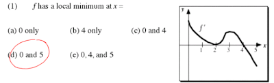
First off, it's obvious that all there really is to this question is to analyze the graph. Still, make sure that you read the question carefully, because it's asking for a LOCAL minimum, which brought up some silly bewilderment today when some of us haphazardly chose their answer without making sure they read the question dutifully enough (this group includes me =/). Now, if you look closely at the graph, we know that since the function in the graph is the derivative of f, in order to determine where f has a local maximum or a local minimum in this case is to analyze the roots of f'.

Knowing the behaviour of the derivative of a function and it's relation to the parent function helps incredibly in this analysis. You must know that not all roots of f' are maximums or minimums, such at x = 2. This is because since there is no sign change, what happens at x = 2 is that there exists a plateau or flat portion in the parent function, thus the horizontal slope at x = 2. Also, looking at x = 4 as another candidate for a local minimum or maximum yields a sign change from positive to negative. This change indicates that x = 4 yields a maximum on the parent function, because since f' is positive to the left of x = 4 and negative to the right of x = 4 the parent function is increasing until it hits x = 4 then turns downwards, therefore it is a local maximum. Now there's only one thing left to analyze since the zero's are now out of the question.

Don't forget about the endpoints of the function. At the endpoints of f', since f is increasing on (0, 4) and then f starts to decrease once again on (4, 5), they turn out to be LOCAL minima on the parent function. This is because since the function start out low at x = 0 and then increases from that point on until x = 4, it is a local minimum. After the function reaches x = 4, the function begins to decrease and therefore reaches another low point at the end of the function. Don't confuse the question with finding the global minimum, which is actually the mistake that I made when I chose my answer. You must recognize that local minima are only considered minima on a small interval central to that point, not over the entire function. Thus both endpoints qualify as LOCAL minima.

Answer: There are local minima at x = 0 and x = 5.

Question #2:

For question number 2, here comes that same graph of f again. But this time we are asked to determine the points of inflection of the parent function f. Though the previous question relied on the endpoints of the function, we cannot do that this time since it's impossible to determine the derivative of the endpoints of a function since there's no one specific derivative at that point. If you imagine trying to draw a tangent line at x = 0 or x = 5 on f', there's no way you can draw just one definite tangent line, thus the illegal procedure of differentiating this function. You might be asking as to why I'm mentioning differentiating this function when it already is the derivative. Recall that we're looking for the inflection point of f, which is a change in the concavity of the function, and that f'' represents the concavity of the parent function, thus the reason for differentiating f'.

We basically are now looking for the zero's of f'', which occur at the local maxima and minima of f'. We can quickly see that there is a maximum present at x = 3 and a minimum at x =2, therefore these are also the points of inflection of f. Don't forget, however, to analyze the shape of these points to determine whether they are in fact points of inflection or not.

Answer: There are points of inflection at x = 2 and x = 3.

Question #3:

In this question, the level of comprehension required for this question does not really bypass the simple rules of antidifferentiating polynomial functions and knowing the connection between acceleration, velocity, and position. This required connection involves the fundamental theorem of calculus, which implicates the process of integration as the reverse of differentiation. Knowing this, and seeing that velocity is defined as a change in position over a given time interval, it can also be perceived as the time derivative of position, which is also followed by the relationship between acceleration and velocity. This indicates that antidifferentiating the acceleration function given gives us the velocity function. But don't forget that the arbitrary constant of integration, C, must be determined using the fact that v(0) = 1. Using this, we can easily solve for C by substituting 0 in for t and setting this equal to 1. Now, since velocity and position are also related similarly, we can antidifferentiate this new velocity function to determine the position function. Don't forget once again, however, to use the fact that s(0) = 3 in order to determine the constants value and finish off the final function.

Answer: s(t) = t³ + t + 3

Question #4:

This question is a truly interesting one, and also sparked a discussion as Mr. K was pulling up the answers to the quiz. It was really just a discussion concerning the negative sign of the cos(x) function, though this quarrel was quickly settled as Mr. K began detailing the solution to the problem. Now on with a reiteration of Mr. K's solution, though I will tend to elaborate wherever I can.

Since we're finding the area under two separate function on the interval x = 0 to x = k, we know that we're going to be finding the value of two separate integrals with the intervals lower and upper limits. Also, just looking at these functions yields should yield a sigh of relief since these functions aren't complicated at all to antidifferentiate each function, so it would be quite easy to continue on that path now. First, as it shows in Mr. K's work, we must set these two integrals equal to each other on the same interval, 0 to k. Then, all you must do is antidifferentiate each function, giving you an equality as shown in the first line in black print in Mr. K's solution above. Don't forget that the antiderivative of sin(x) is -cos(x) and not just cos(x). Remember this is so because the derivative of cos(x) is -sin(x), so just sin(x) is just missing that negative sign when going backwards. Also, don't neglect substituting the 0 into the trigonometric function -cos(x) when integrating the left side, since cos(0) yields a 1. Watch the negative signs though, and try not to get mixed up by the negatives in the function.

Now once you have determined the final equality after antidifferentiating and inserting k and 0, you could solve this in two different ways. You could either leave the two functions equal to each other, and find points of intersection between the two graphs. Or you could find move everything to one side and find the zero's of the function. Either way, it'll require the use of your calculator but yet still yield the same answer.

Answer: 1.300
____________________________________________________________

And now, on to the problem for today's class, the Boston By The Sea" problem. First off, Mr. K quickly told us the origin of Boston as a harbour that slowly grew outwards into the ever-growing city it is now. He really only mentioned that since the question modeled the city using a semi-circle. Here is the question.

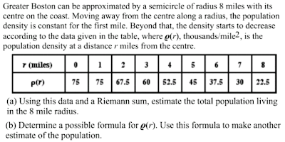
In class, we were only able to cover question (a), though our solution never came to fruition and is therefore homework for Friday's class. Now on to our discussion concerning the first portion of this question.

Now you must first identify what your first task is while approaching this question. If you analyze the question thoroughly, as you should do for long answer questions similar to this, you should notice that the density function gives a value in units of population (in thousands)/miles².
You now must be able to try and find a way to multiply the thousands of people by a unit that will reduce with the miles² to only give the answer a final unit of population (in thousands of people). This can be done by multiplying the density function by the areas of various semi-circles with varying radii. All of our work on this problem can be seen on the following slide

The function in the top left of the above slide depicts the integral Craig proposed to solve the problem part (a). Through much discussion, however, it was decided that this integral would not work for one main reason. The reason is that if we were to use this integral, we would be finding the area of successive semi-circles with changing radii, the further out you go from the center, the larger radii, but this poses a problem because each following area will include the area of the previous semi-circle, meaning you'd be adding the area of each semi-circle several times using this integral. Now we're also going to have to use only the interval given in the data, to find a Riemann sum, but we can only use the intervals of. Therefore, estimating the area underneath the curve (which is the integral we're looking for) would require us to know the values between 0 and 1, 1 and 2, 2 and 3, etc.,but we don't know these values so we can't use left and right-hand sums unless we only use the given data.

Now, follow the yellow section of the figure to the left, and the yellow highlighted function just to the right of the figure as they correspond to each other. Looking at the data, we can see that there is no change in density in the very first semi-circle of radius 1. Thus, we can create a simple expression to show the amount of people in this section by multiplying the density function by the area of this semi-circle. This very expression is what is highlighted in yellow.

But now we must try and model the rest of the semi-circles, and we can do this by breaking each semi-circle into rings between each circumference. One of these rings is represented by the green section in the diagram. This ring can be taken out and straightened out to then be represented by a rectangle, which is also shown by the green highlighted section. The length of this rectangle will be equivalent to the circumference of the semi-circle, and will have a width equivalent to the change in the radius, which is consistently one in this case. Therefore, we now have a model to determine the actual amount of people in the entire section between r = 0 and r = 8. Adding the successive parts of each interval to the expression highlighted in yellow will yield us our final answer for part (a).

Now, our homework for today's class was to finish up this problem and calculate the amount of people in the 8 mile radius. Don't forget to complete your homework for Friday's class everyone.

I think that's all for my scribe post today. As I mentioned in the beginning of my scribe post, the scribe for tomorrow's class will be ETHAN, that is unless he can't make it to class again, in which case the scribe will be VAN. Goodnight everyone and have a pleasant tomorrow! ( I can't remember where that's from, but oh well! =D) I hope my scribe post helped anyone who was in seek of some elaboration upon today's class, or was yearning for some explanation on the subject of applications of integrals. Have a good one everyone!